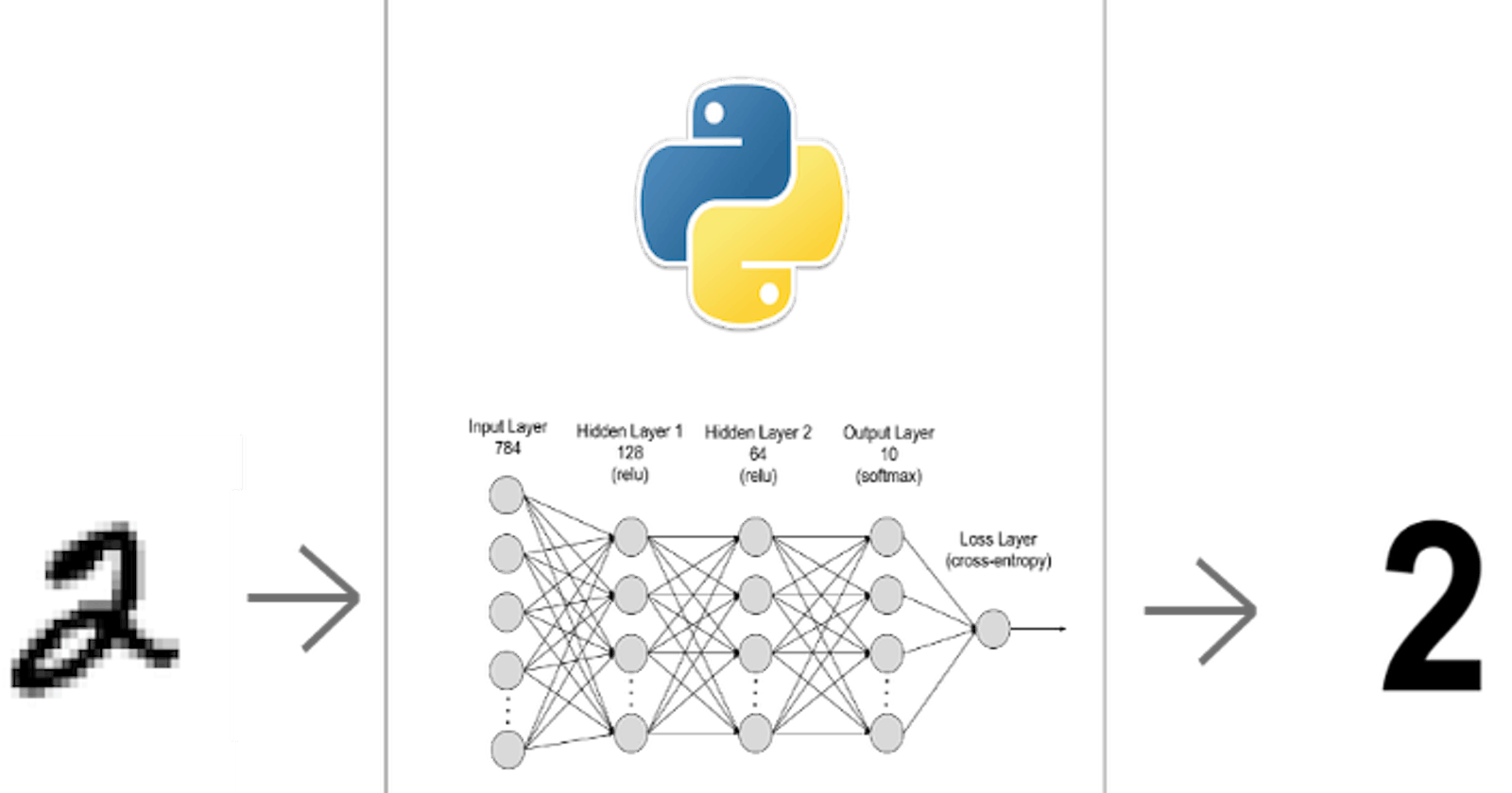
"Smooth Brain" Digit Recognizer Factoid: Machine Learning From Scratch
How feedforward artificial neural network can be used to detect digits... or not?
Table of contents
- Change of plan
- Nodejs vs Django vs Flask vs FastAPI
- How to let users to write with cursors
- How to send the image data to the server
- How to see 👀
- Logistic Regression
- Predict
- Train
- Smooth Brain Neurons
- Neural Network
- Gradient descent for multi-class logistic regression
- Feedforward Neural Network
- Algorithm for 1-hidden layer feedforward neural network
- MNIST handwritten digit dataset
- Deploy!
For a live demo (works on desktop browser): https://digit-recognizer-factoid.herokuapp.com/
I am currently going through #100Devs. If you don't know what it is, make sure to go to twitter and search for #100Devs!! It's an excellent community of people helping each other in their software journey.
Anyways, as part of our assigned work, we had to make a simple calculator:

I finished the calculator, and you can try the working example at: jihoyoo-100devs-calculator.netlify.app
So... that's great!!! But... it's kind of boring and I want to make something a bit more unique to put it into my portfolio. As some of you guys know, I'm a machine learning whizz (not..), so I'm going to make a website where users can go on and be able to write stuff with their cursors. THEN, with some magic, the calculator reads it and spits the answer back out. Basically, I want to put giant eyes to detect digits and symbols to calculate!!
Change of plan
Except, I decided not to do that. Unfortunately, I did not have any datasets for the operations: +, -, /, x. So, I will go with a digit recognizer. Not just any recognizer but it's a factoid! So it'll tell you some facts about the digit you wrote.
I will use this numbers api for the "factoid" part.
Nodejs vs Django vs Flask vs FastAPI
Before going further, I had to choose which framework/environment to use for this project. Since, I recently read: Part III: Build web applications of
I first tried using a Node.js app. But I quickly ran into a problem of having to build a machine learning algorithm in Javascript, and it'd be a nightmare to be doing so many matrix multiplications in JS! Also, numpy is quite efficient in linear algebra due to some magic under the hood. So, I decided to go with a framework that used Python for the sake of my soul😂 Upon searching for Python alternatives, I found Django and Flask to be the most popular, followed by FastAPI which was recommended to me by:
Django seemed a bit too heavy of a tool for what I needed. Hence, I went with lighter framework: Flask or FastAPI. In the end, I went with Flask because I already got started with Flask and it worked. I heard a lot of good feedbacks about FastAPI, so for my next project, I might try FastAPI. My file structure for this project will be:
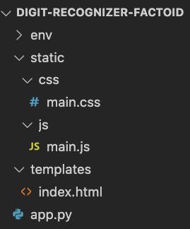
app.py: handles all the routingstatic: holds Javascript and CSS filestemplate: holds HTML
Before getting into the details of the code, let's think about a few engineering challenges:
- How to let users to write with cursors
- How to send the image data to the server
- Machine learning algorithm: How to see 👀
How to let users to write with cursors
I did a bit of searching, and I found out there is a Canvas object in JS which can be used to draw on a canvas.
I struggled to resize the canvas at first, but later I found out that I need to set their size in JS not in CSS. Apparently, setting it in CSS makes the canvas zoom in or out instead. Also, I had to disable scrolling because it was interfering with calculation of finding out the location of the cursor on canvas.
With a little bit of fiddling, I was able to get to this point:
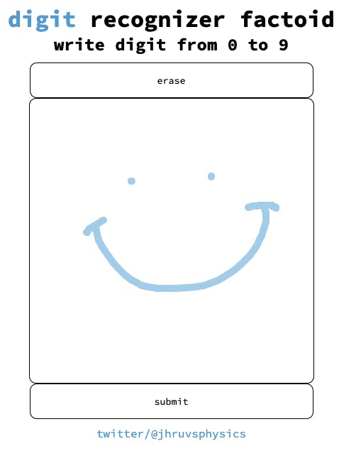
That's it! At least the front-end part of the application is done. Now let's move on to sending this to app.py.
How to send the image data to the server
In main.js, it will handle all the front-end behaviour. Hence, I need a way to send a Canvas object to app.py. This took me a long time to figure out, but this involved the following steps:
Convert Canvas object to Data URI:
image_base64 = canvas.toDataURL('image/jpeg').replace(/^data:image\/jpeg;base64,/, "")Send it via POST request:
fetch('/', {
      method: 'POST',
      body: image_base64
  })
  .then(res => console.log(res))
Receive it from
app.py. Then process base64 to numpy arrayimage = processb64(request.data):def processb64(data): # decode base64 to bytes base64_decoded = base64.b64decode(data) # convert to BytesIO, and open via Image.open image = Image.open(io.BytesIO(base64_decoded)) # resize image = image.resize((28, 28)) # convert to grayscale image gray_image = ImageOps.grayscale(image) image_np = np.array(gray_image) return image_np
I wanted a numpy array of size 28 by 28 representing grayscale image where each location of the element in the array represent pixel-color of an image. This will get sent to the machine learning algorithm for predictions.
By the way, I was going to resize and turn the image into grayscale myself, but thanks to:
I saved a ton of time by simply using the libraries provided by PIL😊
How to see 👀
Now on to the last part and probably the hardest! Train a model to be able to detect digits!!
I am going to use just plain ol' Artificial Neural Network (ANN) to train the model. Convolutional Neural Network seems to be an overkill for this task. This has added benefit of me to being able to write the algorithm from scratch at least in a reasonable amount of time. This is known as supervised learning. In large there are 2 types:
- Regression: predicting a real-vector.
- Classification: trying to predict a category
We are interested in the problem of classification.
WARNING: it involves linear algebra, calculus, and statistics.
Before going into neural networks, let's talk about linear models.
Logistic Regression
Consider a classic problem of binary classification:
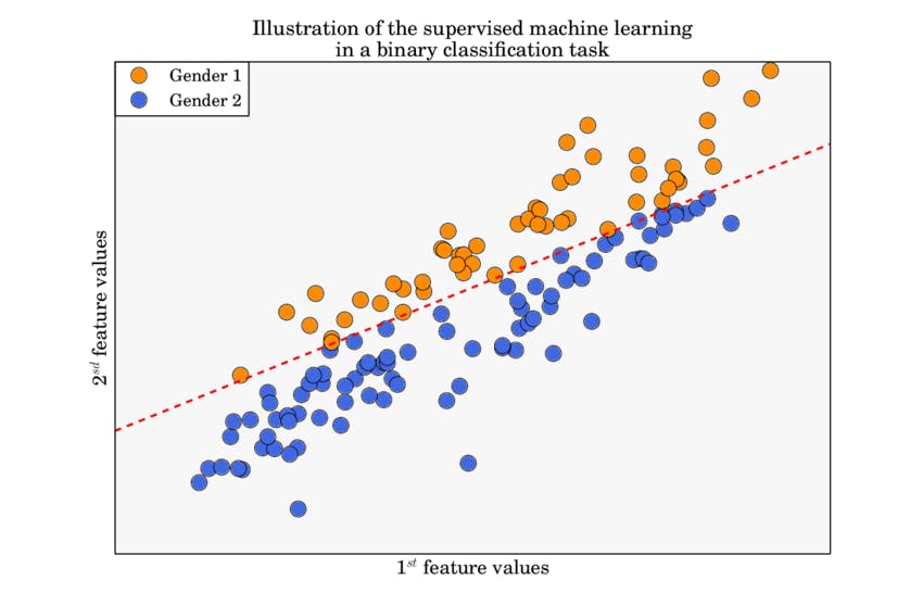
We would like to find the line that clearly separates the two classes. But before jumping into the how to train, let's discuss how to predict.
Predict
Let x = (x1, x2) from the separation line (assume we already trained the model). Assume for some vector w and a real number b,
$$ w^T x + b = 0 \Rightarrow h(x) = w^T x + b $$
Note we are making use of broadcasting rule in Python.
Let class 0 be Gender 2 and class 1 be Gender 1 from our example. Then for some x'=(x'1, x'2), say belonging to class 0, we have h(x')>0 and for some x' belonging to class 1, h(x')<0. However, range of h is not bound, and we would like to have an output in the range [0, 1] where closer to 1 means it's more likely to be in class 1. This is where activation function comes into play:
$$ \sigma(a) = \frac{1}{1 + \exp(-a)} $$
One can check that as a->infinity => σ->1, and as a->-infinity => σ->0.
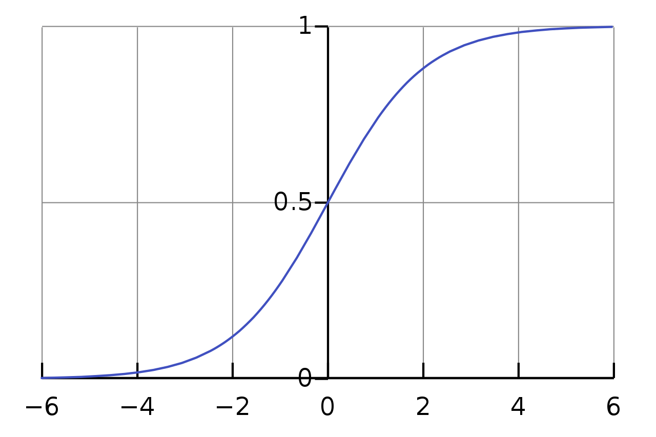
So our output prediction probability can be given by composing the two functions:
$$ probability = \sigma \circ h (w^Tx + b) $$
And we interpret this as probability of x being in class 1.
Train
In order to train the model, we need a cost function to minimize. For binary classification, there is an equation called binary cross-entropy (as a convention we use t for target, the actual class x belongs to, and y for the prediction probability):
$$ J = -\left(\sum_n t_n \log y_n + (1-t_n) \log(1-y_n)\right) $$
Now, it seems like I just pulled this out of a hat. So you may be questioning whether this is actually the best one to use. Good news is that if you are familiar with likelihood function, then you should be able to show minimizing our error function is equivalent to maximizing the likelihood function. In other words, the error function is equivalent to a negative log likelihood. All of these to say that our loss function is fine!
One can check that for t=1 and y=1, J=0. For t=1 and y=0, J=infinity. In order to minimize this, we will use to use gradient descent: $$ w \leftarrow w - \eta \nabla_w J $$ $$ b \leftarrow b - \eta \frac{\partial J}{\partial b} $$
η is called a learning rate and it's a real number. In the above equation, we are basically taking a step in the direction of the gradient because that's where the minimum lies. In the case of J = (w-a)2 for some a, taking the gradient descent will look something like:
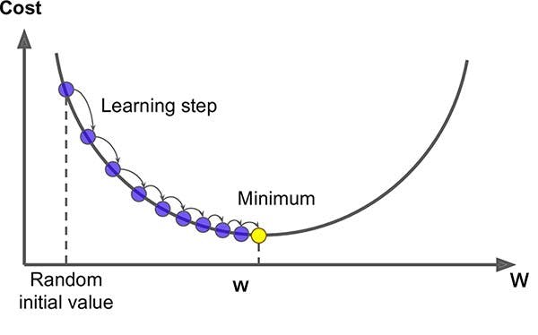
With some work, you should get the following results:
$$ \nabla_w J = X^T(Y-T) $$ $$ \frac{\partial J}{\partial b} = \sum_n (y_n - t_n) $$
where
$$ X = \left( \matrix{ 1 & (\vec x_1)_2 & (\vec x_1)_3 \cr 1 & (\vec x_1)_2 & (\vec x_2)_3 \cr \vdots & \vdots & \vdots \cr 1 & (\vec x_N)_2 & (\vec x_N)_3 \cr } \right) $$
$$ (\vec x_i)_j = j^{th} \ component \ of \ \vec x_i $$
$$ Y = \left( \matrix{ y_1\cr y_2\cr \vdots\cr y_N } \right), \ \ T = \left( \matrix{ t_1\cr t_2\cr \vdots\cr t_N } \right) $$
You can show that
$$ w^Tx + b = Xw $$
Hence
$$ prediction = round(\sigma(Xw)) $$
Putting all of these equations in matrix form is going to benefit us when constructing neural network algorithms.
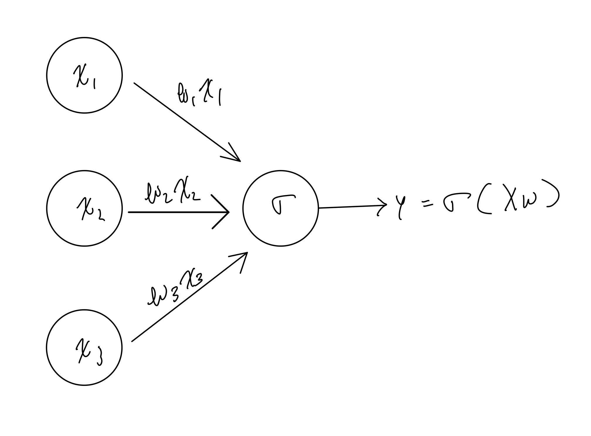
Smooth Brain Neurons
You might ask... where are the neurons? So, I give you one:
Note that x1 is 1 by our construction. Here we see it graphically that xi are multiplied by wi and their total sum is passed to the sigmoid activation function. Its final output is the prediction probability.
With this graph in mind, you should have clearer picture of what our neural networks will be! We will begin to add more neurons and layers.
Neural Network
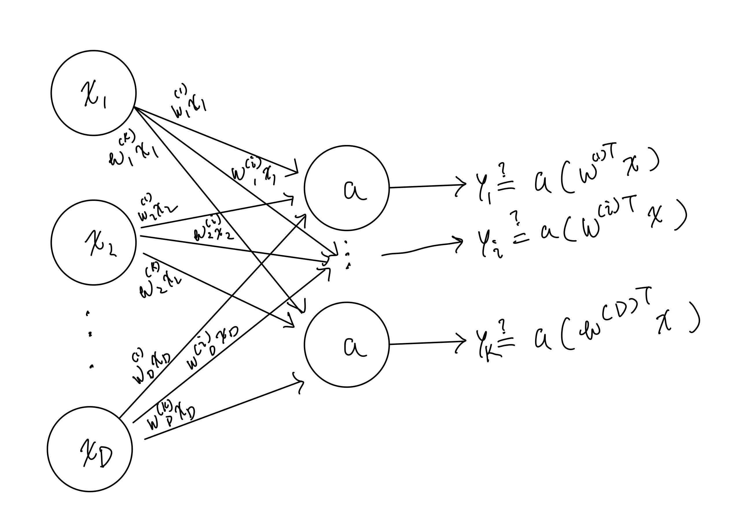
Consider an input x with feature dimension D (dimensionality of x) and K output classes yi we have that
Here, I let wj(i) be weight associated with xj and yi where j=1,2,..., N and i=1,2,..., K.
For such a K-classification, we use categorical cross entropy function J = -Σ n Σ k tnk log(ynk) where tnk (ynk) refers to kth component of nth target (prediction). Note that we use one-hot encoding for target and predictions.
However, we do not know what the activation function is supposed to be. We cannot use sigmoid since we would like
$$ \sum_i y_i = 1 $$
because probability of x belonging to one of K classes is 1. For the activation function, we use softmax
$$ softmax(Xw^{(k)}) = probability(Y=k \vert X) = \frac{\exp(Xw^{(k)})}{\sum_i \exp(Xw^{(i)})} $$
We can further vectorize the equations by letting
$$ X = \left( \matrix{ x_1^T\cr x_2^T\cr \vdots\cr x_N^T\cr } \right), \ \ W = \left( \matrix{ w^{(1)} & w^{(2)} & \cdots & w^{(K)} } \right) $$
Then
$$ Y = \left( \matrix{ y^{(1)T} \cr y^{(2)T} \cr \vdots \cr y^{(N)T} \cr } \right) = softmax(XW) $$
where
$$ y^{(n)} = \left( \matrix{ y_1^{(n)}=softmax(Xw^{(1)})\cr y_2^{(n)}=softmax(Xw^{(2)})\cr \vdots\cr y_K^{(n)}=softmax(Xw^{(K)})\cr } \right) $$
is the nth sample prediction. This is known as multi-class logistic regression.
Gradient descent for multi-class logistic regression
For gradient descent, we need to calculate for (using Einstein notation, repeated indices are summed over) (it's really annoying but hashnode has a bug where it won't display subscript correctly for Latex syntax. So, I'm going to switch to using superscript enclosed by brackets. Wij = W(ij)):
$$ \frac{\partial J}{\partial W^{(ik)}} = \frac{\partial J}{\partial y^{(n k')}}\frac{\partial y^{(n k')}}{\partial a^{(n'j)}}\frac{\partial a^{(n'j)}}{\partial W^{(ik)}} $$
where
$$ J = \sum_n \sum_k J^{(nk)} = \sum_n \sum_k t^{(nk)}\log y^{(nk)} $$
$$ a^{(n'k)} = \sum_\ell X^{(n' \ell)}W^{(\ell k)} $$
But not all of the variables are independent. Above equation is equivalent to (not in Einstein notation): $$ \frac{\partial J}{\partial W^{(ik)}} = \sum_{n, k'} \frac{\partial J^{(n k')}}{\partial y^{(nk')}}\frac{\partial y^{(n k')}}{\partial a^{(n k)}}\frac{\partial a^{(n k)}}{\partial W^{(ik)}} $$
In the end, you should get $$ \frac{\partial J}{\partial W^{(ik)}} = -\sum_n^N (t^{(nk)} - y^{(nk)})x^{(ni)} $$ $$ \nabla_W J = X^T(Y-T) $$
Feedforward Neural Network
We are one layer away from (nontrivial) feedforward neural network! Imagine that outputs from the initial input be input to the next layer, and the next output be the input to the next, and so on. Then, you finally get artificial neural netowrk!
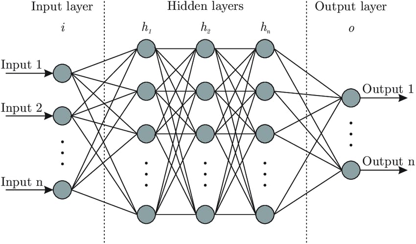
Easy peasy eh? Except, we need to figure out how to do gradient descent:
$$ W \leftarrow W - \eta \nabla_W J $$
Hence, we need to know:
$$ \nabla_W J = \ ? $$
With some help of vector calculus, you should be able to do this calculation (but it's very ugly)! However, in general, above calculation depends on the number of hidden layers. So do we have to calculate this gradient by hand every time we construct a new ANN? Well to a some degree. But you don't have to calculate arbitrary number of terms for arbitrary number of hidden neurons.
So fear not! Luckily for us, we can algorithmically calculate gradients by utilizing backpropagation. It's using chain rules to recursively calculate the derivative starting from the output layer to the previous layer.
Hence, if you are able to construct gradient descents for 2 hidden layer ANNs, there are no more handwritten calculations needed even with more layers added thanks to recursive nature of chain rule.
Algorithm for 1-hidden layer feedforward neural network
We are basically done with theoretical introduction to neural network. Now, let's make 1-hidden layer feedforward neural network. This will be used to classify digits.
Consider input X (NxD), hidden layer Z(NxM), and output Y(NxK) => N samples with M hidden neurons. Then, W (DxM) and b (M) are the weights for X, and V (MxK) and c (K) are the weights for Z. The bracket indicates their dimensionality. Notice that we did not absorb b and c into the weight matrix.
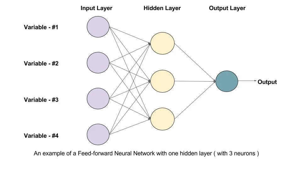
For the above example, we have D=4, M=3, K=1. Let's calculate (1-sample) gradient descent. Let
$$ Z = \sigma(\alpha) = \sigma(XW + b) $$ $$ Y = softmax(a) = softmax(ZV+ c) $$ $$ J = \sum_n \sum_k t^{(nk)}\log y^{(nk)} $$
Then
$$ \frac{\partial J}{\partial V^{(mk)}} = \sum_n^N\sum_q^K \frac{\partial J^{(nq)}}{\partial y^{(nq)}} \frac{\partial y^{(nq)}}{\partial a^{(nk)}} \frac{\partial a^{(nk)}}{\partial V^{(mk)}} = \sum_n^N (y^{(nk)} - t^{(nk)})z^{(nm)} $$ $$ \frac{\partial J}{\partial c^{(k)}} = \sum_n^N\sum_q^K \frac{\partial J^{(nq)}}{\partial y^{(nq)}} \frac{\partial y^{(nq)}}{\partial a^{(nk)}} \frac{\partial a^{(nk)}}{\partial c^{(k)}} = \sum_n^N (y^{(nk)} - t^{(nk)}) $$
And
$$ \frac{\partial J}{\partial W^{(dm)}} = \sum_k^K\sum_n^N\sum_q^K \frac{\partial J^{(nq)}}{\partial y^{(nq)}} \frac{\partial y^{(nq)}}{\partial a^{(nk)}} \frac{\partial a^{(nk)}}{\partial z^{(nm)}} \frac{\partial z^{(nm)}}{\partial \alpha^{(nm)}} \frac{\partial \alpha^{(nm)}}{\partial W^{(dm)}} $$ $$ \Rightarrow \frac{\partial J}{\partial W^{(dm)}} = \sum_k^K \sum_n^N (y^{(nk)} - t^{(nk)})V^{(mk)}z^{(nm)}(1-z^{(nm)})x^{(nd)} $$ $$ \frac{\partial J}{\partial b^{(m)}} = \sum_k^K\sum_n^N\sum_q^K \frac{\partial J^{(nq)}}{\partial y^{(nq)}} \frac{\partial y^{(nq)}}{\partial a^{(nk)}} \frac{\partial a^{(nk)}}{\partial z^{(nm)}} \frac{\partial z^{(nm)}}{\partial \alpha^{(nm)}} \frac{\partial \alpha^{(nm)}}{\partial b^{(m)}} $$ $$ \Rightarrow \frac{\partial J}{\partial b^{(m)}} = \sum_k^K \sum_n^N (y^{(nk)} - t^{(nk)})V^{(mk)}z^{(nm)}(1-z^{(nm)}) $$
In vector form:
$$ \nabla_V J = Z^T(Y-T) $$
$$ \nabla_W J = X^T \left[ [(Y-T)V^T]⊙Z' \right] $$
where
$$ Z' = Z⊙(1-Z) \ for \ sigmoid \ activation $$
where ⊙ is component-wise sum
With this, now I have everything there is to create feedforward neural network with 1 hidden layer.
MNIST handwritten digit dataset
Note, this is 1 layer neural network (no hidden layer)
I am going to be using MNIST dataset for training my model for digit classification. Getting the data is as easy as
from tensorflow.keras.datasets import mnist
(Xtrain, Ytrain), (Xtest, Ytest) = mnist.load_data()
In order to process this image data, we first have to flatten the data since it's 28x28 per sample. Then our feature dimension D=784. Also, we one-hot encode the targets. Also, we normalize the data.
def flatten(X):
  # This will flatten the last two indices
  # if [[a, b], [c, d]] -> [a, b, c, d] per sample
  N, dim1, dim2 = X.shape
  return X.reshape(N, dim1*dim2)

def onehot(Y):
  K = np.max(Y)+1
  return np.eye(K)[Y]
Ytest_ind = onehot(Ytest)
Ytrain_ind = onehot(Ytrain)

Xtest = flatten(Xtest)
Xtrain = flatten(Xtrain)

# normalize the data
mu = Xtrain.mean(axis=0)
std = Xtrain.std(axis=0)

idx = np.where(std == 0)[0]
assert(np.all(std[idx] == 0))

np.place(std, std==0, 1)

Xtrain = (Xtrain-mu)/std
Xtest = (Xtest-mu)/std
We initialize the weights:
# Initialize weights
W = np.random.randn(D, K)/np.sqrt(D)
b = np.zeros(K)
The gradient descent step:
# gradient descent
d_WJ = Xtrain.T.dot(P_Y - Ytrain_ind)
d_bJ = np.sum(P_Y - Ytrain_ind, axis=0)
W -= learning_rate*d_WJ
b -= learning_rate*d_bJ
After training for 2500 epochs (iterations), the cost for the train and test dataset is:
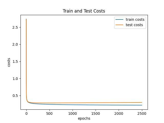
Unfortunately, although this worked quite well on MNIST dataset which was quite surprising, the accuracy wasn't satisfactory on the canvas images. I suspect it may have had difficult time due to translational variance. This could be solved via some fancy image processing techniques, or by using an architecture similar to LeNet that uses Convolutional Neural Network with Pooling layers. It tries to find many different patterns/features of different sizes relevant to the categorization irrespective of where it is located. Hence, I did not bother with 1 hidden layer neural network, instead I implemented the LeNet-like CNN architecture by utilizing a library. All the codes, including the smooth brain neural network, will be available in Github
Deploy!
I am going to deploy this app via Heroku. This took considerable amount of time since I've never used anything other than netlify to host my website. I had issues with regards to passing HTTP request instead of HTTPS request. Therefore, I made my own API as a proxy to the original API and hosted it on Heroku.
For a live demo (works on desktop browser): https://digit-recognizer-factoid.herokuapp.com/
Conclusion
Phew! That was a lot of work but I really enjoyed making it. I spent good amount of time outside of the algorithm itself, but rather on figuring out how to deploy my application on the web. In the future, I'd like to explore more on machine learning theories, algorithms, and its applications. Specifically, I would like to cover topics on Convolutional Neural Network. I am also interested in Reinforcement learning, and many others.
If you enjoyed my content, please consider following me! I love putting my work out there and more people the better! :)
